1.6. Illustrations numériques autour de la méthode du rejet

1.6.1. Exemple: loi gamma par la méthode du rejet

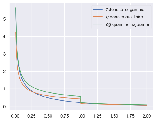
Soit \(\alpha \in ]0, 1[\). On considère \(X\) de loi gamma de paramètre \(\alpha\) i.e. de densité

\[\begin{equation*} f(x) = \frac{1}{\Gamma(\alpha)} x^{\alpha - 1} e^{-x} \mathbf{1}_{]0,+\infty[}(x). \end{equation*}\]

Pour mettre en oeuvre la méthode du rejet on considère par exemple la densité auxiliaire

\[\begin{equation*} g(x) = \frac{\alpha e}{\alpha + e} \big(x^{\alpha-1} \mathbf{1}_{]0,1[}(x) + e^{-x} \mathbf{1}_{[1,+\infty[}(x) \big) \end{equation*}\]

qui vérifie \(f(x) \le \big(\frac{\alpha + e}{\alpha e \Gamma(\alpha)} \big) g(x)\) pour tout \(x \in \mathbf{R}\). Il est très important de considérer les fonctions \(f\) et \(g\) normalisées c’est à dire telles que \(\int f(x) \operatorname{d}\! x = \int g(x) \operatorname{d}\! x = 1\). La constante qui apparait dans l’hypothèse de majoration est donc ici \(c_\alpha = \frac{\alpha + e}{\alpha e \Gamma(\alpha)} > 1\).

Pour simuler selon la loi de densité \(g\) on utilise l’inverse de la fonction de répartition: on vérifie que la fonction quantile \(G^{-1}\) s’écrit

\[\begin{equation*} \forall u \in ]0,1[, \quad G^{-1}(u) = \big(\frac{\alpha + e}{e} u \big)^{1/\alpha} \mathbf{1}_{\{u < \frac{e}{\alpha+e}\}} - \log \big((1-u) \frac{\alpha + e}{\alpha e} \big) \mathbf{1}_{\{u \ge \frac{e}{\alpha + e}\}}. \end{equation*}\]

import numpy as np
import scipy.stats as stats 
from scipy.special import gamma
import matplotlib.pyplot as plt
import seaborn as sns
sns.set_theme()

alpha = 0.5
rv = stats.gamma(alpha)

x = np.linspace(0.01, 2, 1000)

# toujours écrire une fonction vectorielle 
# c'est à dire qui s'applique à un argument x de type `numpy.array`
# il faut donc éviter les tests `if x < 1 else ...`
def g(x, alpha): 
    cst = (alpha * np.exp(1)) / (alpha + np.exp(1))
    result = np.empty_like(x)
    result[x < 1] = x[x < 1]**(alpha-1)
    result[x >= 1] = np.exp(-x[x >= 1])
    return cst * result
    
# la constante c de l'hypothèse de domination 
c = (alpha + np.exp(1)) / (alpha * np.exp(1) * gamma(alpha))

fig, ax = plt.subplots(1, 1)
ax.plot(x, rv.pdf(x), label=r'$f$ densité loi gamma')
ax.plot(x, g(x, alpha), label=r'$g$ densité auxiliaire')
ax.plot(x, c*g(x, alpha), label='$cg$ quantité majorante')
ax.legend()

<matplotlib.legend.Legend at 0x16abcfb90>

1.6.2. Exemple: lien avec une méthode intuitive pour la loi uniforme